Marginal Propensity to Consume

• NOTE: I wrote this last night, before I read this morning’s Letters From an American, where Heather Cox Richardson wrote about this topic.

As the new administration starts to finalize its plans for the coming years – excuse me, the concepts of its plans – we’ll start hearing a lot about tax cuts. I want to talk a little today about how all tax cuts are not the same.

In the 1980s, the Reagan administration drastically altered the tax code in the United States.

In the 1950s, the top marginal income tax rate was 91% for incomes over $200,000 (about $2 million in today’s dollars), the average effective tax rate for the top 1% was 42%, and the average effective tax rate for all households was 17% (The marginal income tax rate is the percentage you pay on the last dollar of income earned. This concept is central to progressive tax systems, where tax rates increase as income rises.)

By the end of the 1980s, the top marginal tax rate was 50% for incomes over $100,000, while the average effective tax rate for the top 1% was 28% and the average effective tax rate for all households was around 14%.

This was supposed to fuel supply-side economic growth; producers would invest their new-found wealth in business expansion, creating jobs and putting money in people’s pockets. The people would in turn look for ways to spend their money, placing greater demands on producers who would then produce even more, build even more, hire even more, and so forth. This was called “trickle-down” economics. The decrease in income tax revenue from the wealthy would be offset by increased income tax revenue paid by the millions of workers in their new jobs. Instead of putting money directly in people’s hands as the US had done since the New Deal, this was supposed to be a more sustainable process of stimulating economic growth.

The problem, of course, was that it didn’t work. Instead of investing in the domestic economy, the rich people used their money to purchase houses in the Bahamas, buy expensive foreign-made cars, and fund stock buy-backs that put money in the hands of stockholders and corporate executives rather than the workers. The businesses didn’t expand, the new jobs weren’t created, and the federal deficit soared.

I won’t go through the history of the efforts of every Republican president since Reagan (that means Bush and Trump) to use the same playbook – with the same results, budget deficits, and economic crisis.

This is all because of an economic concept called the “Marginal Propensity to Consume.” This is an economic metric that quantifies the proportion of additional income that a consumer will spend on goods and services, as opposed to saving it.

Low-income people (LIPs) have a higher marginal propensity to consume (MPC) than high-income people (HIPs) for several reasons (LIPs and HIPs are my invention because I got tired of typing the same words over and over):

• LIPs need to allocate a larger portion of their income to cover essential living expenses. Any additional income is quickly spent on these necessities, which may be the result of pent-up demand or needed improvement in their quality of life.

• LIPs generally have lower savings and fewer financial assets and are not in the habit of saving or investing. They will spend any additional income to improve their immediate living conditions.

• LIPs have limited access to credit, making them more dependent on current income for their current needs.

• LIPs experience greater satisfaction from additional income than HIPs do. Going out to dinner, for example, means a lot more for a LIP than a HIP.

The policy implications for this are clear. A tax cut for LIPs, who have a higher propensity to consume, is going to result in a more immediate and substantial boost in consumer spending. This generates greater demand for goods and services, leading to higher economic growth and potentially creating more jobs. Such tax cuts would also provide LIPs with more disposable income, potentially allowing them to move away from government-funding income support programs and toward self-sufficiency. This has ripple effects throughout their families, as family members have better access to education, health care, and employment, keeping the cycle moving upward.

A tax cut for HIPs, on the other hand, results in more savings and a smaller increase in consumer spending. HIPs are less likely to spend this increase on immediate needs but rather might invest it in businesses or stocks. This can contribute to economic growth but more slowly and less directly than increased consumer spending. Because tax cuts for HIPs primarily benefit people who are already well-off, they lead to greater economic disparity over time.

We don’t have to wait and see what the impact of the tax cuts Trump is proposing in his second term. He’s done this before, in his Tax Cuts and Jobs Act of December 2017. Although this bill generated a small increase in GDP, it was not as great as initially projected. Real wages increase, but more slowly than GDP and more pronounced for HIPs. The Corporate Tax Rate (capital gains) was permanently reduced from 35% to 21%, and revenues from corporate taxes fell by almost half.

The result was a significant increase in the federal deficit and the national debt. The deficit (the yearly calculation of the difference between revenue and expenditures) increased 17% in 2018 (the first year the new tax rates were in effect) and 11% in 2019. The deficit for 2020 was huge, primarily due to COVID, but began to decrease in the succeeding years. The anticipated extension of the Trump tax cuts would add $4.6 trillion to the deficit while producing a $112.6 billion windfall for the top five percent of income earners in the first year alone. You can check out the Senate Budget Committee Report that provides this information here.

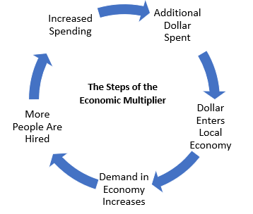
We need to introduce two more terms to make sense of this – the circular flow of income and the Multiplier effect. The circular flow of income assumes that the recipient of money from any transaction will spend that money in some fashion (depending on their marginal propensity to consume), which generates new income for someone else, which generates further new spending, and so forth. The multiplier says that the total increase in final income will be some level greater than the new injection to spend. Mathematically, the multiplier effect is the inverse of the marginal propensity to consume.

Here's an example of how this works: Let’s assume an average MPC of 80% and an initial expenditure of $1,000 paid to a police officer.

• The officer spends 80% of this ($800) on a plane ticket to Hawaii.

• The owner of the airline spends 80% of this ($640) on a new office computer.

• The owner of the computer store spends 80% of this ($512) on an advertising billboard.

I won’t carry this out any further, but here’s how GDP increased more than the original $1,000. The additional increase adds up to; $1,952 ($800 +$600+$512). The cycle continues until there’s only an insignificant of money that could be spent.

There’s a joke in here somewhere about dieting which includes “a minute on the lips, forever on the hips” but I can’t make it work this morning.